Team Introduction
Bringing together drone enthusiasts to create the extraordinary through technology
Newest Drone Lineup
Generations of self-developed and iterated drone platforms
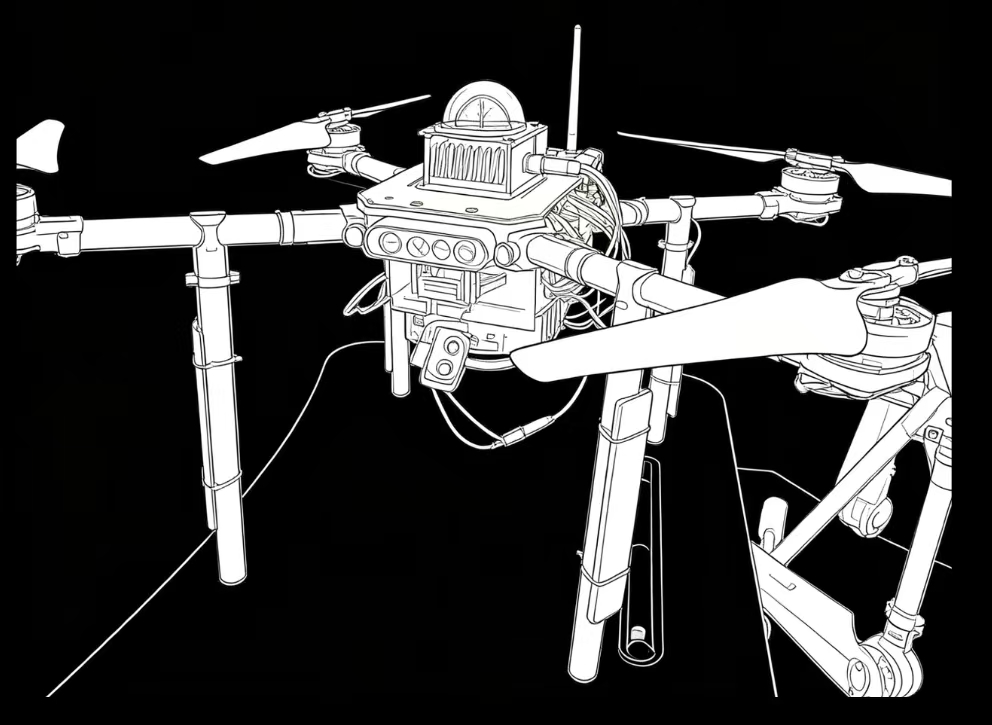
SUAS2026 Drone
Drone for SUAS competition 20261-kilogram payload capacity and is designed to perform autonomous target recognition, object delivery, and 2D mapping tasks.
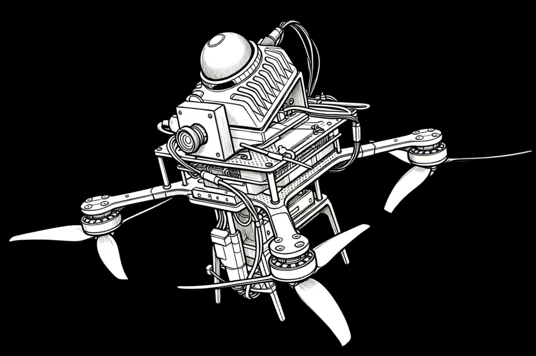
Drone for MTR Inspection Project
Drone for MTR Inspection ProjectLiDAR-based autonomous drones feature obstacle-avoidance capabilities in dense environments and the ability to generate 3D semantic maps.
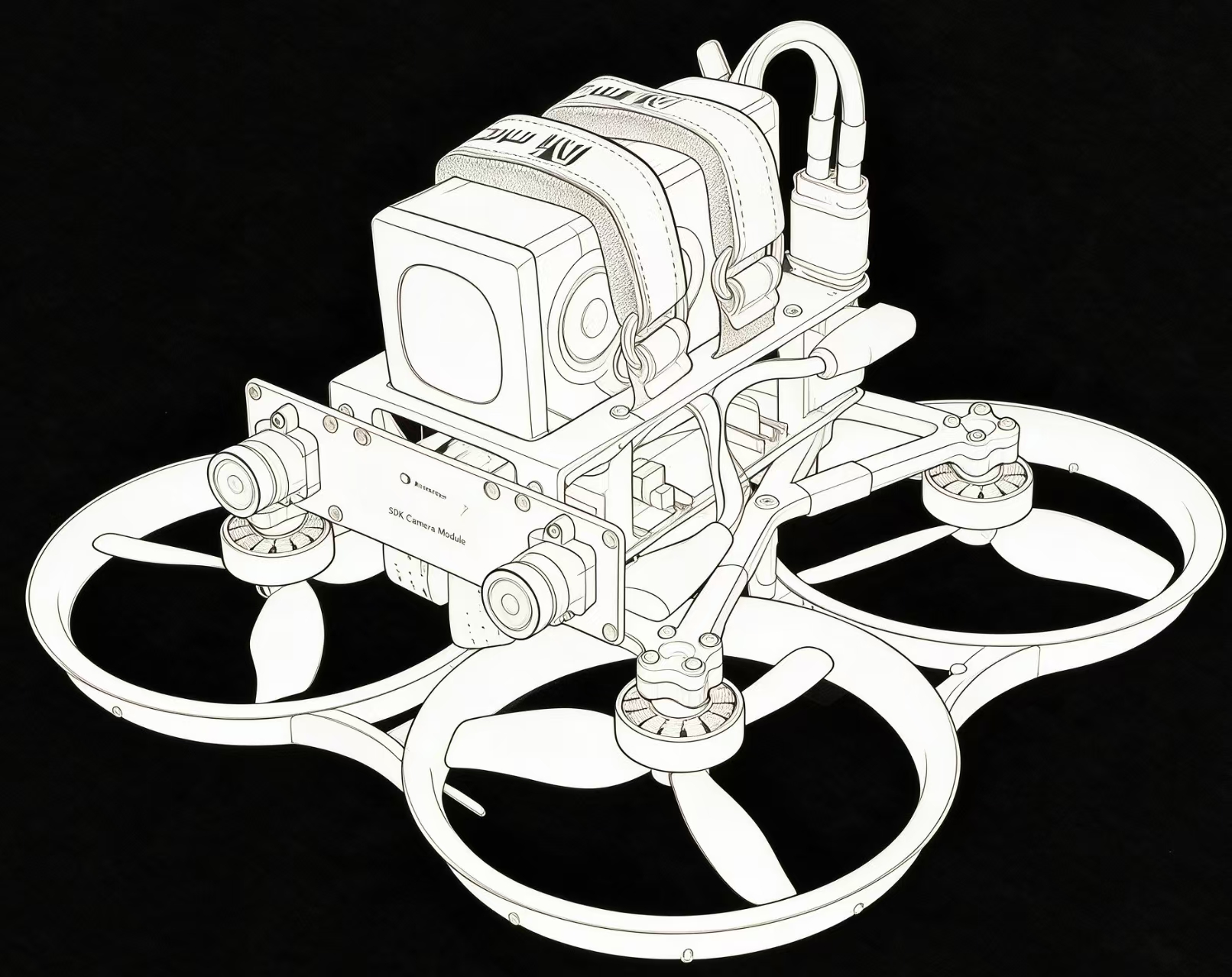
Drone for NN-based Planning
Drone for NN-based Planning ProjectEmploy neural-network-based obstacle avoidance, with optimization performed on the onboard NPU
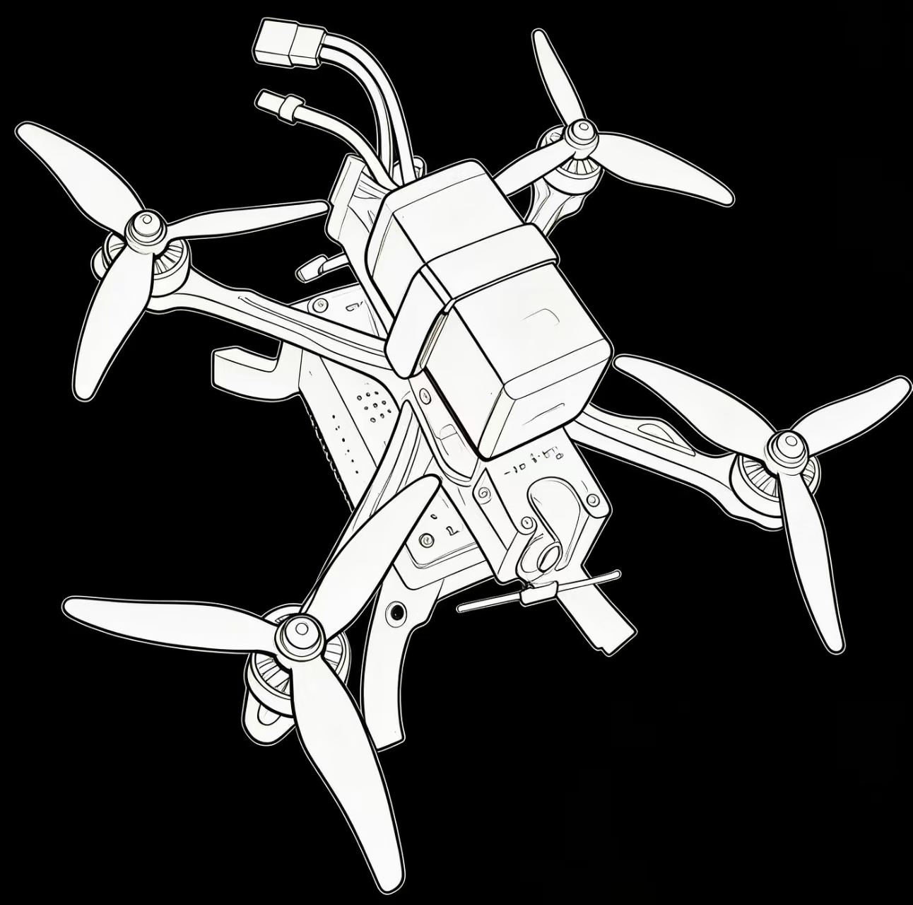
Drone for RL-based flight control
Drone for RL-based flight controlHigh-Maneuver Flight Control Based on Reinforcement Learning
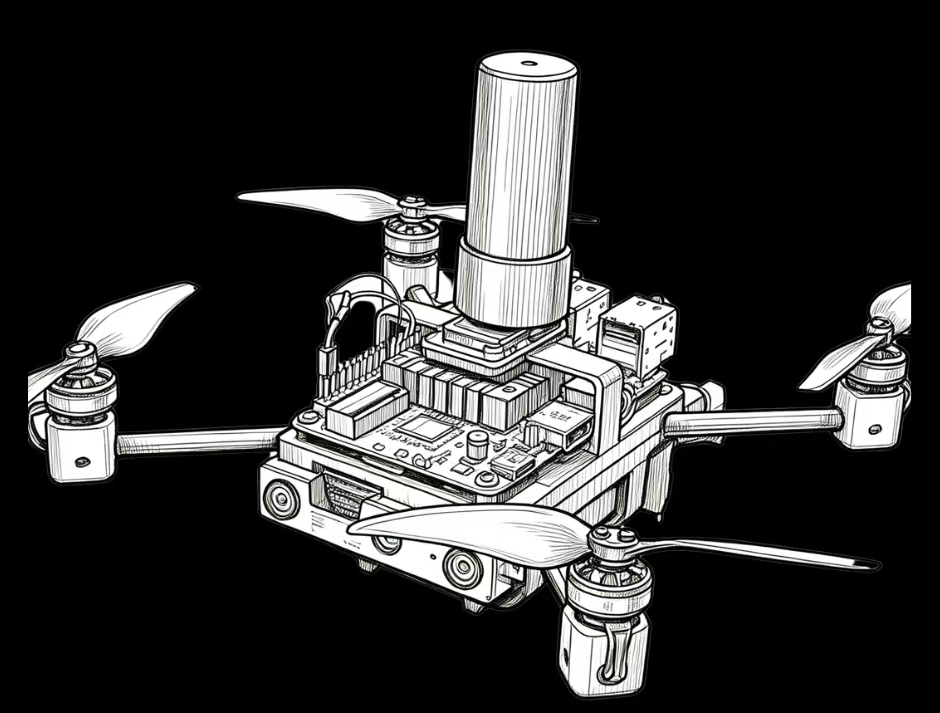
Drone for IARC Competition
Drone for IARC Competition 2026-2027equipped with a swarm-based unknown-environment coverage algorithm and 2D mapping capabilities.
Our Team
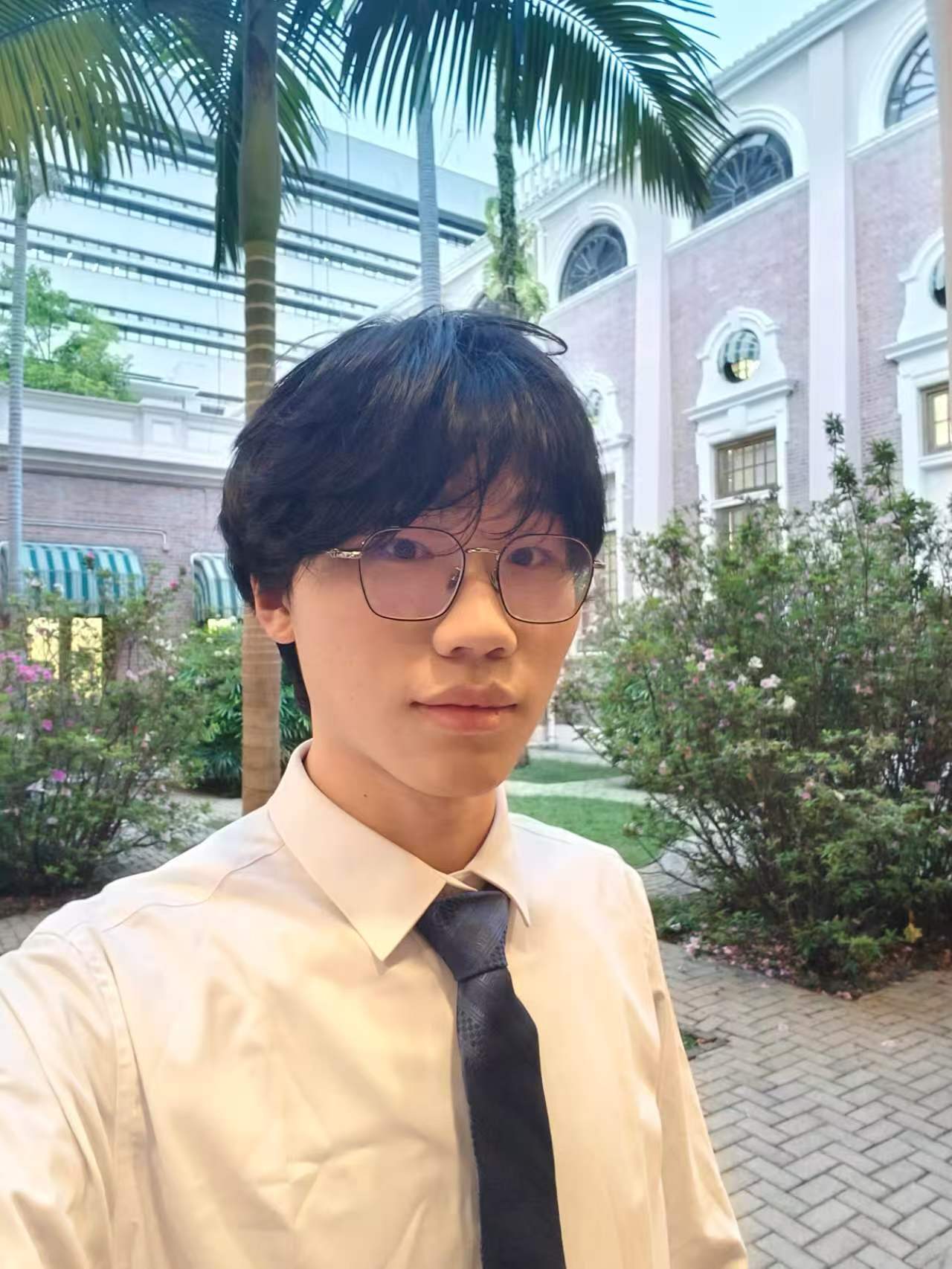
Oscar
Computer Engineering · PlannerOversees overall project planning and planner algorithm research

Alex
Mechanical Engineering · StructuresSpecializes in airframe structural design and powertrain optimization
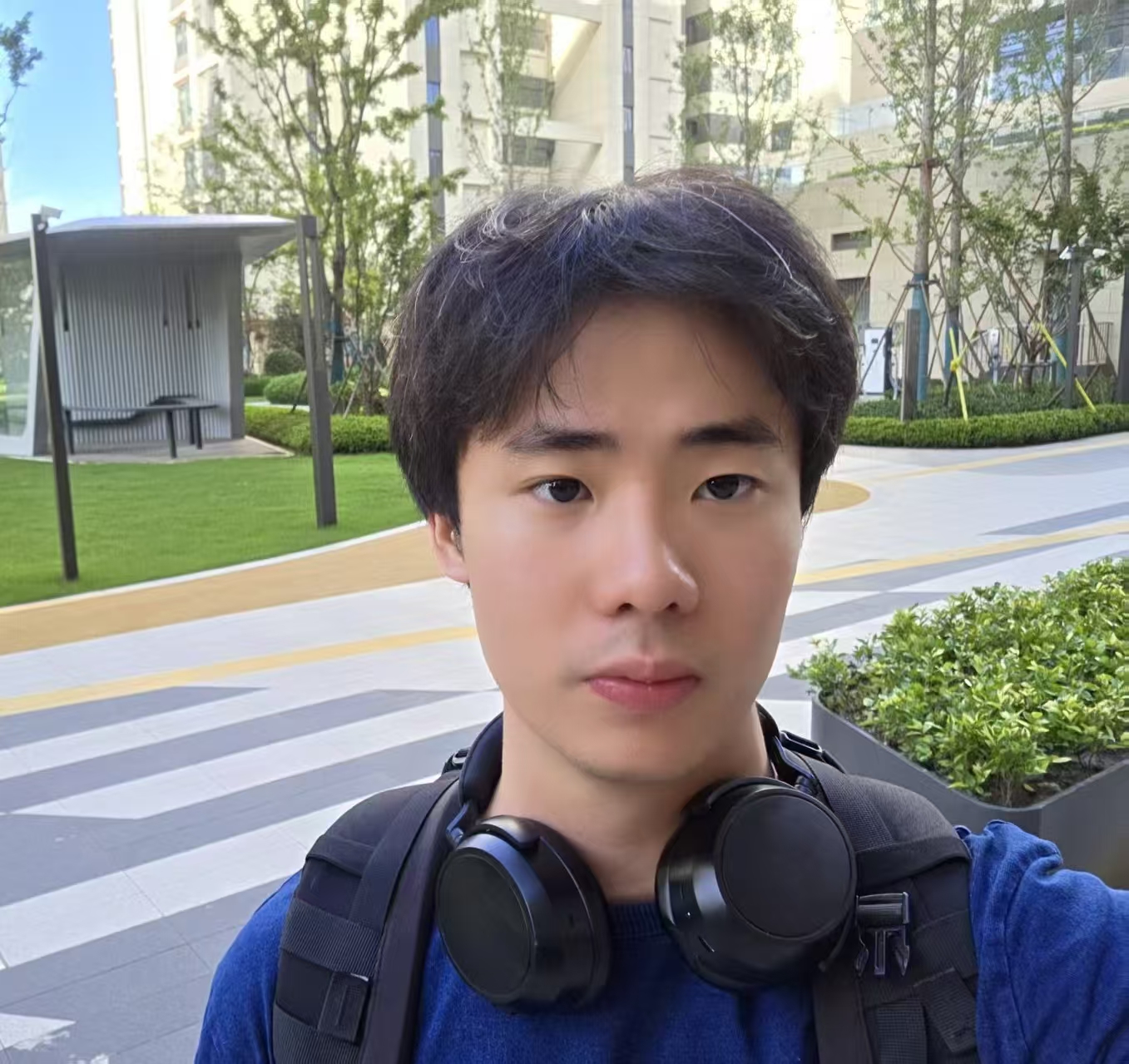
Henry
Computer Science · Flight ControlResponsible for flight/Motion control and computer vision algorithm development

Ilyas
Electrical Engineering · Communication & MCUResearches UAV communication links, flight controller chips
Activities & Achievements
Constantly pushing boundaries in competitions and in the lab
SUAS Competition
winnerSUAS competition 2021, 2022, 2023
Final Year Project
runner-upFinal Year Project 2020, 2021, 2022, 2023, 2024, 2026
MTR Drone Project
doneMTR Drone Project 2025, 2026
HKU-THU Drone Project
doneHKU-THU Drone Project 2025
Inno Show
doneInno Show 2020, 2021, 2022, 2023, 2024
Student Interest Course
doneStudent Interest Course 2025, 2026
Current Work
Core research topics and engineering projects in progress

IARC Competition 2026-2027
IARC Competition Mission 10, About using a swarm drone system for Mines Detection and Mapping in Unknown Areas
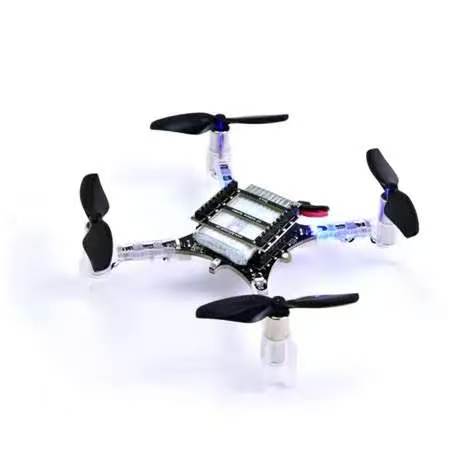
Crazyflie Swarm System
Based on Motion Capture Technology or Lighthouse System to control a swarm of Crazyflie drones and form a pattern
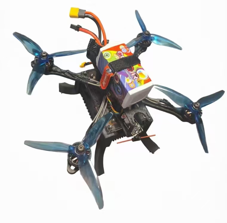
RL-based Control System
Investigating the application of reinforcement learning algorithms for autonomous control of drone swarms in dynamic environments
Drone Guide
A complete drone learning path from the ground up — covering hardware, flight control, ROS2, simulation, and environmental perception
Common Drone Classifications
- Multirotor: Quadcopters, hexacopters, octocopters — most common for hobby and research. Excellent hovering capability and vertical take-off/landing. Ideal for close-range inspection, aerial photography, and indoor operations.
- Fixed-Wing: Long endurance (often 1-4 hours), high cruise speed — suitable for large-area aerial surveying, agricultural monitoring, and long-range delivery. Requires runway or catapult launch.
- VTOL (Vertical Take-Off & Landing): Combines the hovering capability of multirotors with the efficiency of fixed-wing aircraft. Can take off vertically then transition to forward flight.
- Single-Rotor Helicopter: One main rotor plus tail rotor — higher payload capacity and longer endurance than multirotors of similar weight. Mechanically more complex.
Key Terminology
- Flight Controller (FC): The "cerebellum" of the drone — a dedicated microcontroller running real-time firmware (PX4/ArduPilot) that handles attitude stabilization, position control, and motor output.
- ESC (Electronic Speed Controller): Receives low-voltage PWM signals from the FC, amplifies them via gate drivers, and switches MOSFETs to deliver high-voltage three-phase power to brushless motors.
- IMU (Inertial Measurement Unit): Combines accelerometers and gyroscopes to measure linear acceleration and angular velocity. Essential for attitude estimation.
- PID Controller: Proportional-Integral-Derivative control algorithm — the fundamental method for stabilizing drone attitude and position.
- Onboard Computer: A companion computer (e.g., Raspberry Pi, Jetson Nano/Orin) that handles high-level tasks like vision processing, path planning, and ROS2 communication — separate from the real-time FC.
A drone can be decomposed into three major subsystems:
1. Power Components
- Brushless DC Motors: Outer-ring rotor design for higher torque and better heat dissipation. Key parameter: KV rating (RPM increase per volt of input). Lower KV (~900) for larger props, higher KV (~2000+) for smaller/faster setups.
- ESC (Electronic Speed Controller): Converts DC battery power into three-phase AC for the motor. Modern ESCs support protocols like DShot for digital, high-speed communication.
- Battery: Typically LiPo (Lithium Polymer) — specified by cell count (e.g., 4S = 14.8V nominal) and capacity (mAh). Higher voltage = more power; higher capacity = longer flight.
- Propellers: Come in CW/CCW pairs. Diameter and pitch determine thrust characteristics.
2. Computer (Brain)
- Flight Controller (FC): The real-time "cerebellum" that runs PID loops at 250Hz-4kHz. Reads sensors (IMU, GPS, barometer), computes attitude, and outputs motor commands via PWM.
- Onboard Computer: Handles computationally heavy tasks — computer vision, SLAM, path planning, ROS2 nodes. Communicates with the FC via UART (typically TELEM port) using MAVLink protocol.
3. Sensors
- IMU (Accelerometer + Gyroscope): Core attitude sensor — measures linear acceleration and angular velocity.
- GPS/Compass: Provides global position and heading reference.
- Barometer: Altitude estimation via atmospheric pressure.
- Vision Sensors: Cameras, LiDAR, depth sensors for advanced perception.
Multirotor drones achieve various flight maneuvers by adjusting the speed differences between motors. The flight controller computes a target state (desired position, orientation, attitude, thrust) and compares it with the current state measured by sensors. The error drives motor commands:
- Throttle (Up/Down): Increase/decrease all motor speeds simultaneously to generate more or less total thrust.
- Roll (Left/Right tilt): Speed up motors on one side, slow down the other — creates a torque around the front-back axis.
- Pitch (Forward/Back tilt): Speed difference between front and rear motors — creates torque around the left-right axis.
- Yaw (Rotation): Speed up CW motors while slowing CCW motors (or vice versa) — exploits counter-torque to rotate around the vertical axis.
The transformation from desired position (x, y, z) and orientation (φ, ω, κ) down to individual motor PWM signals goes through multiple cascaded PID loops: Position → Velocity → Attitude → Rate → Motor Mixer → PWM.
Coordinate Frames
- Body Frame: Origin at the drone's center of gravity. X-axis points forward (nose direction), Y-axis points right, Z-axis points down. Sensor readings are in this frame.
- World/NED Frame (North-East-Down): Fixed to the Earth. X points North, Y points East, Z points Down (toward Earth center). GPS coordinates are referenced here.
- ENU Frame (East-North-Up): Alternative world frame — X East, Y North, Z Up. Common in ROS and computer vision.
Attitude Representations
- Euler Angles (Roll φ, Pitch θ, Yaw ψ): Intuitive three-angle representation. Drawback: suffers from gimbal lock at pitch = ±90°.
- Rotation Matrix (SO(3)): 3×3 orthogonal matrix. 9 numbers to represent 3 DOF — redundant but unambiguous.
- Quaternions: 4-element representation (w + xi + yj + zk). No gimbal lock, computationally efficient for chaining rotations. The standard in PX4, ROS, and most flight control software.
Brushless DC Motors
Drones use outer-ring rotor brushless motors where the outer casing rotates around fixed internal windings. This design provides higher torque and better heat dissipation compared to inner-rotor designs.
- KV Rating: Speed per volt — for every 1V increase in input, the motor's no-load RPM increases by KV. Lower KV (500-1000) for large propellers; higher KV (2000-3000) for small/fast setups.
- Three-Phase Operation: The ESC sequentially energizes pairs of the three windings (AB → AC → BC → …), creating a rotating magnetic field that pulls the permanent-magnet rotor.
- Direction Reversal: Swap any two of the three motor wires to reverse rotation direction.
ESC (Electronic Speed Controller)
The ESC receives low-voltage PWM signals from the flight controller, processes them, and drives MOSFETs to deliver high-voltage three-phase power:
- Microcontroller reads the PWM duty cycle from the FC
- Gate driver amplifies the low-voltage control signal
- MOSFETs switch high-current battery power to the motor phases
PWM Duty Cycle: As the PWM duty cycle increases from 50% to 100%, the effective voltage delivered to the motor increases, causing it to spin faster.
Battery Selection
- LiPo (Lithium Polymer): High discharge rates, lightweight. Cell nominal voltage = 3.7V. Common: 3S (11.1V), 4S (14.8V), 6S (22.2V).
- C-Rating: Maximum safe discharge current = Capacity × C-rating. Example: 5000mAh 30C = 150A max.
Flight Controller (FC) — The "Cerebellum"
The FC is a real-time microcontroller (typically STM32-based) dedicated to low-latency flight-critical tasks:
- Runs PX4 or ArduPilot firmware on an RTOS (NuttX/ChibiOS)
- Executes PID control loops at 250Hz–4kHz
- Reads IMU, barometer, magnetometer, GPS at high frequency
- Outputs PWM/DShot signals to ESCs
- Communicates with onboard computer via UART (TELEM port) using MAVLink
Key FC sensors onboard: IMU (accelerometer + gyroscope), barometer, magnetometer (compass). External: GPS module, rangefinder, optical flow sensor.
Onboard Computer — The "Cerebrum"
A Linux-based companion computer (Raspberry Pi, Jetson Nano/Orin, Intel NUC) handling computationally intensive tasks:
- Runs ROS2 nodes for path planning, SLAM, object detection
- Processes camera/LiDAR data (OpenCV, PyTorch, etc.)
- Connects to FC via UART/USB (MAVLink or MicroXRCEAgent)
- May include a dedicated GPU/NPU for neural network inference
Why Can't We Combine Them?
Real-time flight control requires deterministic sub-millisecond timing that a Linux OS cannot guarantee. Separating the real-time FC from the high-level onboard computer ensures that critical stabilization loops are never interrupted by CPU-intensive vision or planning tasks.
MEMS IMU (Micro-Electro-Mechanical System)
Modern drone IMUs are fabricated on silicon chips using MEMS technology, integrating both a 3-axis accelerometer and a 3-axis gyroscope in a tiny package.
MEMS Gyroscope — Measuring Angular Velocity
Uses the Coriolis force principle:
- A flexible micro-oscillator is driven to resonate at ~14 kHz along one axis
- When the sensor rotates, the Coriolis force deflects the oscillator perpendicular to both the vibration and rotation axes
- Capacitive sensors detect the deflection amplitude
- Coriolis acceleration = 2 × (ω × mass_velocity), from which ω (angular rate) is derived
MEMS Accelerometer — Measuring Linear Acceleration
Uses a micro-flexible hinge with a proof mass:
- A micro-hinge is fabricated on silicon allowing deformation in the detection direction
- When acceleration occurs, the proof mass shifts relative to fixed electrodes
- Capacitive sensing measures the displacement
- F = ma → acceleration magnitude is computed
6-Axis IMU: 3-axis gyro + 3-axis accelerometer. 9-Axis IMU: adds 3-axis magnetometer (compass).
Recommended Setup (Entry-Level F450 Quad)
| Component | Recommended Model | Key Specs |
|---|---|---|
| Frame | F450 | 450mm wheelbase, glass-fiber arms, classic entry frame |
| Flight Controller | Pixhawk 2.4.8 / CUAV V5+ | STM32F4/F7, dual IMU, supports ArduPilot/PX4 |
| Motor | 2212 920KV | Outer-rotor brushless, pairs with 10-inch props |
| ESC | 30A BLHeli_S | Supports DShot300/600 digital protocol |
| Battery | 4S 5200mAh LiPo | ~20 min hover, 30C+ discharge rate |
| GPS+Compass | M8N GPS / Here3 | Dual GNSS, external compass, safety switch |
| Transmitter | RadioMaster TX16S | OpenTX/EdgeTX, multi-protocol module, 16 channels |
| Receiver | FrSky X8R / ELRS 2.4G | SBUS/PPM output, telemetry capable |
- Frame Assembly: Attach four arms to the base plate. Install landing gear. Ensure all screws are thread-locked but not overtightened.
- Motor Mounting: Mount motors on arm ends with M3 screws. Route motor wires along arms toward the center.
- ESC Installation: Solder ESCs to the power distribution board (PDB) or place on arms. Connect ESC signal wires to FC PWM output pins (Motor 1-4).
- FC Mounting: Mount the FC on vibration-dampening standoffs. The arrow on the FC MUST point toward the nose (forward direction). Connect IMU, barometer internally.
- GPS/Compass: Mount on a mast away from EMI sources (ESCs, power wires). Connect to FC GPS/I2C port. Observe correct orientation.
- Receiver Wiring: Connect receiver SBUS/PPM output to FC RC input. Bind with transmitter before powering on.
- Propeller Installation: CW prop on CW motors, CCW prop on CCW motors. Use nylon lock nuts. Double-check direction — incorrect prop installation is the #1 cause of maiden flight failure.
- Final Check: Verify all connections, check COG (should be centered), confirm no loose wires near props, verify motor rotation directions via FC motor test.
PX4 Architecture
PX4 is an open-source flight control firmware running on NuttX RTOS. Its two core software components:
- Control Loops: Cascaded PID control loops for position, velocity, attitude, and rate — all running on the real-time FC processor (see the Control tab for detailed control theory).
- EKF2 (Extended Kalman Filter): Fuses data from IMU, GPS, magnetometer, barometer, optical flow, and vision sensors to produce a consistent state estimate (see the Perception tab for detailed estimation theory).
Both control and estimation run directly on the flight controller hardware (STM32 processor), ensuring real-time performance.
QGroundControl (QGC) — Ground Station
QGC is the primary ground control station for PX4-based drones. Key functions:
- Firmware Flashing: Flash PX4 firmware to the FC via USB.
- Sensor Calibration: Calibrate accelerometer, gyroscope, compass, and level horizon with guided wizards.
- Radio Calibration: Map transmitter channels and set endpoints.
- Flight Mode Setup: Configure Stabilize, Altitude, Position (Loiter), Mission, Return, Offboard modes.
- PID Tuning: Adjust rate and attitude PID gains in real-time with live plotting.
- Mission Planning: Draw waypoint missions on a satellite map; upload to drone.
- Failsafe Configuration: Set low-battery RTL, RC loss, geofence, and data link loss actions.
- Telemetry View: Real-time flight data — attitude, altitude, GPS, battery, and sensor health.
Why Do We Need ROS?
Scenario: You have a drone with a LiDAR. You want it to move forward and stop in front of a wall.
If you write everything in one file: read LiDAR hardware port → detect range → make decision → send command to FC... you face problems:
- A second file also needs LiDAR data — but the hardware port is already occupied!
- Read, logic, and control are entangled — you can't test or replace them individually.
- What about systems spanning multiple machines (onboard computer + FC) and networks?
You'd think: "Write a separate LiDAR reader, distribute messages via queue/pipe/shared memory." And for multi-machine: "Use TCP/UDP." But for incredibly large and complex systems, configuring all this manually is extremely inconvenient. This is why we need ROS.
What is ROS2?
ROS2 is a communication middleware built on top of DDS (Data Distribution Service). DDS handles all the complexity of distributed communication — ROS2 further simplifies DDS usage by providing a clean API. Your code just calls simple publish/subscribe functions; ROS2 handles everything underneath.
DDS Core Concepts
DDS is primarily data-driven communication middleware. Data transmission is handled by DataReader/DataWriter, with QoS (Quality of Service) controlling transmission quality (reliability, durability, deadline, etc.). ROS2 inherits all properties of DDS.
ROS2 Communication Methods
- Node: Your code/file — e.g., a LiDAR reader or logic processor. Each node is an independent process.
- Topic: The message title/channel name. Nodes publish/subscribe to named topics.
- Message (msg): The data structure sent over a topic (e.g., sensor_msgs/Image, geometry_msgs/Twist).
- Publisher: Sends messages to a topic. Many nodes can publish to the same topic.
- Subscriber: Receives messages from a topic. Many nodes can subscribe to the same topic — each message is broadcast to all subscribers.
- Service (srv): Request-Response pattern. Client sends a request, Server processes and sends a response. Multiple clients, one server.
- Action: For long-running tasks. Consists of three parts: Goal (what to do), Feedback (progress updates), Result (final outcome). Supports cancellation.
Essential ROS2 CLI Commands
| Command | Usage |
|---|---|
ros2 run <pkg> <node> | Run a node from a package |
ros2 node list | List all active nodes |
ros2 node info <node> | Show node details (pub/sub, services) |
ros2 topic list | List all active topics |
ros2 topic echo <topic> | Print messages published on a topic |
ros2 topic info <topic> | Show topic type and publishers/subscribers |
ros2 topic pub <topic> <msg> | Publish a message from CLI (no node needed) |
ros2 interface show <type> | Display message/service/action structure |
ros2 service list | List all active services |
ros2 service call <srv> <data> | Call a service from CLI |
colcon build | Build ROS2 workspace packages |
rqt_graph | Visualize node-topic connection graph |
ROS2 Workspace Structure
- Create workspace:
mkdir -p ~/ros2_ws/src && cd ~/ros2_ws - Create package:
ros2 pkg create --build-type ament_python my_package - Write node files: Publisher/Subscriber/Server/Client Python or C++ files
- Configure package.xml: Declare dependencies
- Configure CMakeLists.txt / setup.py: Build configuration
- Build:
colcon build - Source:
source install/setup.bash - Run:
ros2 run my_package my_node
ROS2 Plugins
- rmw (ROS Middleware): DDS implementation layer. Default: CycloneDDS or FastDDS. Can be optimized for 5G and WiFi.
- rosbag2: Record and playback ROS2 topic data — essential for debugging and dataset collection.
- rviz2: 3D visualization tool for sensor data, robot models, and trajectories.
- rqt: Plugin-based GUI toolkit (plot, graph, console, parameter tuning).
The Bridge Problem
PX4 uses uORB (micro Object Request Broker) as its internal messaging system, while ROS2 uses DDS. These are different communication middlewares — we need a bridge to translate between them.
MicroXRCEAgent — The Bridge
PX4 automatically activates all uORB topics when powered on. The MicroXRCEAgent (also called uXRCE-DDS) runs on the onboard computer and bridges uORB ↔ DDS, making PX4 topics available as ROS2 topics.
Offboard Control Flow
Two kinds of information are needed for drone control:
- Target/Flight Point: Where you want the drone to go — sent from ROS2 → PX4 via topics like
/fmu/in/trajectory_setpoint - Current State: Where the drone actually is — published by PX4 → ROS2 via topics like
/fmu/out/vehicle_odometry
To control the drone in Offboard mode:
- Download the PX4 ROS2 message definitions and demo code from the PX4 GitHub
- Start MicroXRCEAgent to bridge PX4 ↔ ROS2
- Publish trajectory setpoints at ≥ 2Hz (or the drone will failsafe)
- Subscribe to vehicle state topics for feedback
- Use
VehicleCommandservice to arm, takeoff, land, and change flight modes
Pre-Flight Simulation Testing is Essential
If you want to build a drone, simulation testing before actual flight is essential. It allows you to:
- Test flight control algorithms without risking hardware damage
- Validate path planning and obstacle avoidance in diverse environments
- Train reinforcement learning policies safely at accelerated speed
- Debug sensor fusion and state estimation with ground truth data
Simulator Comparison
- Gazebo (now Gazebo Harmonic/Ignition): Native ROS2 integration via ros_gz bridge. The best choice for drone development — PX4 provides complete simulation environments. Supports physics, sensors, and multi-vehicle scenarios.
- Omniverse Isaac Sim: Very high-fidelity rendering and physics. Complex setup, best for visual AI training.
- Unreal Engine / AirSim: Photo-realistic rendering. Lacks native ROS2 interface; requires custom bridging.
Team Recommendation: Use Gazebo with PX4 SITL (Software In The Loop).
SDF (Simulation Description Format)
SDF is an XML-based format for describing simulation objects. The four main element types:
- <world>: Describes the complete simulation environment — physics engine settings, gravity, lighting, and all models within it.
- <model>: Describes a robot or object — includes links (rigid bodies), joints (connections), sensors, and plugins.
- <actor>: A special model type for executing scripted animations (e.g., walking pedestrians).
- <light>: Describes lighting sources (point, directional, spot).
Getting SDF Files for Your Robot
- CAD → URDF → SDF: Export your CAD model (SolidWorks/Fusion 360) to URDF using
sw_urdf_exporter, then convert URDF to SDF. - Write xacro files: Use xacro (XML macros) for parameterized robot descriptions, then process into URDF/SDF.
- Gazebo Model Database: The Gazebo project provides a large library of pre-built SDF models (furniture, buildings, roads, sensors).
Setup PX4 Simulation Environment
PX4 has provided a complete simulation environment. To get started:
- Clone the PX4-Autopilot repository:
git clone https://github.com/PX4/PX4-Autopilot.git --recursive - Run the setup script:
bash ./PX4-Autopilot/Tools/setup/ubuntu.sh - Build and launch simulation:
make px4_sitl gazebo
Simulating Different Vehicles
Change the vehicle type by specifying the airframe:
- Quadcopter (default):
make px4_sitl gazebo - Standard VTOL:
make px4_sitl gazebo_standard_vtol - Fixed-Wing: Use appropriate airframe configuration
Simulating Different Worlds
Gazebo worlds define the environment. PX4 includes several:
- Default (empty): Open field with ground plane
- Baylands: Outdoor environment with runways
- Warehouse: Indoor environment for inspection testing
- Custom worlds: Create your own SDF world files with obstacles, buildings, and terrain
Multi-Vehicle Simulation
PX4 also supports multi-vehicle simulation for swarm testing. Each vehicle runs its own PX4 instance with unique MAVLink IDs and UDP ports, all within a single Gazebo world.
Connecting ROS2 to PX4 SITL
With MicroXRCEAgent running, the simulated drone's PX4 topics become available as ROS2 topics — identical to real hardware. This means you can develop and test your entire ROS2 control stack in simulation before deploying to a real drone.
Why Do We Need State Estimation?
Getting correct position and velocity is very difficult because:
- Sensor Noise: All sensors (IMU, GPS, barometer) have random measurement noise.
- Nonlinearity: Sensor observations have significant nonlinear characteristics.
- Multiple Sensors: We have more than one sensor measuring overlapping states — how do we fuse them optimally?
The solution: KF (linear systems) → EKF (nonlinear systems)
Kalman Filter Core Concepts
The robot has a state (e.g., position + velocity). We don't know the actual values; there are many possible combinations. KF assumes each variable follows a Gaussian distribution ℕ(μ, σ²): mean μ is the most likely state, variance σ² quantifies uncertainty.
State Representation
The state at time k is represented by two quantities:
x̂k ∈ ℝn (best estimate), Pk ∈ ℝn×n (covariance matrix)
Covariance Matrix & Correlation
Position and velocity are correlated: high velocity → likely moved far; slow → likely didn't move much. This correlation is captured in the covariance matrix P — each element Pij = Cov(xi, xj) represents the joint uncertainty between state variables i and j. Off-diagonal terms encode this cross-information.
Step 1 — Prediction (Model-Based)
Use the system's motion model Fk and control input uk to predict the next state:
x̂k|k−1 = Fk · x̂k−1 + Bk · uk
Pk|k−1 = Fk · Pk−1 · FkT + Qk
where Qk is the process noise covariance — it captures external disturbances (wind, motor vibrations, modeling errors). Adding Qk inflates the uncertainty to account for unmodeled effects.
Step 2 — Update (Measurement-Based)
Incorporate sensor measurement zk with measurement model Hk and sensor noise R:
ỹk = zk − Hk · x̂k|k−1 (innovation / measurement residual)
Sk = Hk · Pk|k−1 · HkT + R (innovation covariance)
Kk = Pk|k−1 · HkT · Sk−1 (Kalman Gain)
x̂k = x̂k|k−1 + Kk · ỹk
Pk = (I − Kk · Hk) · Pk|k−1
Understanding the Kalman Gain Kk
Kk = PpredHT / (HPpredHT + R). Two extreme cases:
- R → 0 (very accurate sensor): Kk → H−1 — trust the measurement almost entirely.
- Ppred → 0 (very confident prediction): Kk → 0 — ignore the measurement, trust the model.
K elegantly solves: "Given two Gaussian distributions (prediction and measurement), what's the most likely true state?" — it's the weighted overlap (product) of the two Gaussians, with weights determined by their relative uncertainties.
EKF — For Nonlinear Systems
Real drone dynamics are nonlinear: xk+1 = f(xk, uk) + wk, zk = h(xk) + vk. EKF linearizes at the current estimate:
Fk = ∂f/∂x |x̂k−1 (state transition Jacobian)
Hk = ∂h/∂x |x̂k|k−1 (measurement Jacobian)
Then apply the standard KF prediction/update equations using these Jacobians. PX4 uses EKF2 to fuse IMU (250+ Hz), GPS (5-10 Hz), magnetometer, barometer, optical flow, and vision data into a consistent, high-rate state estimate on the FC in real-time.
The Essence of Intelligence is Feature Learning
Humans recognize letters through 2D features, objects through 3D features, motion through 4D features (3D + time), and mathematical relationships through higher-dimensional features. In the past, engineering tried to use hand-crafted features to replicate functions — but the world is far too complex. Some features may never be fully understood by humans.
The Core Mathematical Insight
The core approach to feature extraction is: define a basis function, then perform a dot product between that basis function and your data. This separates features by measuring how much of each basis function is present.
1D Example — Sound Frequency Decomposition
Treat each frequency (sin x, sin 2x, sin 3x…) as an axis of a coordinate system. A sound signal is a vector in that system. By dot-product with each basis function axis, you obtain the coefficients (how much of each frequency is present). Convolution solves the time-alignment problem (the signal may start at different times).
2D Convolution — Image Features
Same principle applied to images. The basis functions are small matrices (e.g., 3×3 kernels). Convolution solves the position problem (features may appear anywhere in the image). Through years of experience, people have discovered useful kernel patterns: edge detectors (Sobel), corner detectors, blob detectors (LoG).
3D & 4D Convolution
3D Convolution: Applied to volumetric data (e.g., CT scans, point cloud voxels). 4D Convolution: 3D + time — for video understanding and spatio-temporal features. Transformer (Attention): Extends this idea to language and other domains — self-attention as learned dot-product feature extraction.
From Hand-Crafted to Learned Features: Neural Networks
How do we know which features are important? Historically, people defined them arbitrarily (e.g., VIO feature detectors). The results were unsatisfactory until neural networks emerged. Humans delegate the "find useful features" process to machines via gradient descent. As layers deepen, features become features of features — from edges → textures → object parts → full objects. When layers get too deep to design, fully connected networks emerged, though they're being replaced by specialized architectures (CNN, Transformer, GNN).
Why Object Detection Matters
For all animals, 2D object detection is crucial — especially for birds that must spot prey from high altitudes. For drones, object detection enables target recognition, obstacle avoidance, search and rescue, and autonomous landing.
YOLO (You Only Look Once)
YOLO is a real-time object detection system that treats detection as a single regression problem —直接从图像像素到边界框坐标和类别概率. It's widely used due to its speed-accuracy balance.
Team Application: Mines Detection
The team has prepared custom datasets for mines detection as part of the IARC competition. Using PyTorch (GPU or CPU version), we train YOLO models to detect and classify target objects from drone camera feeds. This integrates with the ROS2 perception pipeline: Camera → YOLO Node → Detection Topic → Planner Node → Offboard Control.
Sensor Types for Depth Sensing
- LiDAR: Most traditional method — active laser ranging
- Stereo Camera: Two cameras, similar to human eyes — passive triangulation
- Monocular Depth Estimation: Single camera using learned depth cues — AI-driven
LiDAR (Light Detection And Ranging)
Three main measurement methods:
- dTOF (Direct Time-of-Flight): Measures round-trip time of laser pulse. Best for long range.
- iTOF (Indirect Time-of-Flight): Measures phase shift of modulated continuous wave. Better for indoor/short range.
- Triangulation: Uses geometry of laser emitter, target, and receiver. Highest accuracy at very close range.
LiDAR types by scanning mechanism: Mechanical (rotating assembly), MEMS semi-solid-state (micro-mirror), rotating mirror, Flash (illuminates entire scene at once).
Stereo Camera — Stereo Matching
The core challenge: finding corresponding points in two images (the stereo matching problem).
Traditional Approaches:
- Sparse Matching (Feature-based): Match only prominent keypoints (SIFT, ORB, SURF). Fast and robust, but only sparse depth points.
- Dense Matching: Compute disparity for every pixel:
- Local Methods (Block Matching): Fast, real-time (SAD, SSD). Error-prone in low-texture/occlusion areas.
- Semi-Global Methods (SGM): Mainstream in industry/autonomous driving. Balances accuracy and speed with good edge preservation.
- Global Methods: Highest accuracy (Graph Cuts, Belief Propagation). Computationally expensive.
Neural Network Approach — PSMNet: Instead of hand-crafted feature matching, PSMNet uses a CNN to learn stereo matching end-to-end — from image pair to dense disparity map.
Monocular Depth Estimation
Using a single camera with deep learning to estimate depth from monocular cues (texture gradient, occlusion, relative size, perspective). While less accurate than stereo or LiDAR, it's lightweight and cost-effective for certain applications.
What is VIO?
VIO fuses data from camera and IMU sensors to achieve "complementary advantages":
- Camera: Rich visual information, slow drift, but sensitive to motion blur, low texture, and lighting changes. Low update rate (30-60 Hz).
- IMU: High update rate (100-1000 Hz), robust to visual conditions, but suffers from rapid drift when integrated alone.
Together: IMU provides short-term motion prediction (bridging camera blind spots during fast motion), while camera provides long-term drift correction (constraining IMU bias estimates).
Fusion Methods
- Loosely Coupled: Process visual and inertial measurements independently, then fuse their output results (e.g., position, pose). Simpler but less accurate.
- Tightly Coupled: Jointly optimize the residual factors of raw camera features and pre-integrated IMU measurements in a single optimization. Higher accuracy. IMU integration can predict feature locations to accelerate feature tracking and enhance stability in high-dynamic scenarios.
VINS-Fusion
A state-of-the-art tightly-coupled VIO framework supporting stereo+IMU and mono+IMU configurations. Widely used in drone research for GPS-denied navigation.
Beyond VIO
Other advanced perception methods the team explores:
- Occupancy Networks: Learn a continuous 3D occupancy function — represents scene geometry implicitly, enabling novel view synthesis and dense reconstruction.
- 3D Object Detection: Detect and localize objects in 3D space from point clouds or multi-view images. Essential for autonomous navigation.
The Planning Problem
Given a map of the environment (from perception) and a goal, the planner must compute a collision-free, dynamically feasible trajectory from start to goal. For drones, this is a high-dimensional problem: position (3D) + yaw (1D) + time.
Search-Based Planning: A* and Variants
A* (A-Star) is the classic grid-search algorithm that finds the shortest path by combining actual cost-to-come g(n) with heuristic cost-to-go h(n):
f(n) = g(n) + h(n)
- Hybrid A*: Extends A* to continuous state spaces with kinodynamic constraints — generates smooth, executable paths respecting the drone's motion model.
- Lattice Planner: Pre-computes motion primitives (short, feasible trajectory segments) and searches over them — guarantees dynamic feasibility by construction.
Sampling-Based Planning: RRT & PRM
- RRT (Rapidly-exploring Random Tree): Grows a tree from the start by randomly sampling the space and connecting to the nearest node. Probabilistically complete — will find a path if one exists. RRT* adds rewiring for asymptotic optimality.
- PRM (Probabilistic Roadmap): Pre-builds a graph of collision-free configurations offline, then queries it online. Good for static environments with repeated queries.
Gradient-Based Planning: EGO-Planner
EGO-Planner (ESDF-free Gradient-based local Planner) is a state-of-the-art method for aggressive drone flight:
Instead of building an explicit Euclidean Signed Distance Field (ESDF), it computes collision costs directly from the obstacle point cloud and back-propagates gradients to deform a B-spline trajectory away from obstacles:
minQ J = λsJsmooth + λcJcollision + λfJfeasibility
where Q is the B-spline control points, Jsmooth penalizes acceleration/jerk, Jcollision pushes the trajectory away from obstacles via gradient descent, and Jfeasibility enforces velocity/acceleration limits.
- Key Advantage: No ESDF computation needed — works directly on raw point clouds at very high speed (milliseconds per replan).
- Autonomous Replanning: Continuously replans during flight — ideal for dynamic environments and unknown obstacle fields.
Kinodynamic & Differential Flatness
Quadrotors are differentially flat: the full state (position, velocity, attitude, angular velocity) can be expressed as functions of the flat outputs (x, y, z, yaw) and their derivatives. This means we can plan in the 3D position space and recover the full orientation later — dramatically simplifying the planning problem.
The Exploration Problem
When a drone enters an unknown environment, it must simultaneously map and decide where to go next to maximize information gain — trading off exploration (visiting new areas) vs. exploitation (thoroughly mapping known regions).
Frontier-Based Exploration
The classic approach: frontiers are boundaries between known-free and unknown space. The drone greedily navigates to the nearest (or largest) frontier, updates the map, and repeats until no frontiers remain.
- Nearest Frontier: Fast but shortsighted — may miss efficient global coverage.
- Largest Frontier: Prioritizes large unknown regions — better global coverage.
- Cost-Utility: Balances travel cost vs. expected information gain — frontier selection as a utility maximization problem.
Next-Best-View (NBV) Planning
A more sophisticated approach: generate candidate viewpoints, evaluate each by expected information gain (how many unknown voxels become visible), and select the one maximizing gain / travel_cost. NBV naturally handles 3D structures like building facades and bridges that frontier methods miss.
Information-Theoretic Exploration
Treats the occupancy map probabilistically. Each grid cell has entropy (uncertainty):
H(cell) = −pocc log pocc − pfree log pfree
A ray cast through cells reduces their entropy. The expected Information Gain of a candidate viewpoint is the sum of entropy reductions along all its potential rays. This provides a principled, mathematically grounded approach to exploration — especially important for the IARC competition's unknown-environment coverage task.
What are VLA Models?
Vision-Language-Action (VLA) models are a new paradigm that unifies perception, reasoning, and control into a single model. A VLA takes visual input (camera feed) and natural language instruction (e.g., "fly through the window and land on the red table"), and outputs actions directly.
Architecture
VLA models typically combine three components:
- Vision Encoder: A pre-trained vision transformer (ViT) or convolutional backbone that encodes RGB images into a latent representation.
- Language Encoder: A large language model (LLM) that tokenizes and encodes the natural language instruction.
- Action Decoder: A policy head that maps the fused vision-language representation to control actions — either as discrete tokens (via VQ-VAE action tokenization) or continuous regression outputs (waypoints, motor commands).
at = πθ(ot, L)
where ot is the visual observation at time t, L is the language instruction embedding, and at is the action.
Key Capabilities for Drones
- Instruction Following: "Circle around the red building" — the model understands spatial relationships from language alone.
- Zero-Shot Generalization: Trained on diverse data, VLAs can handle novel objects and commands never seen during training.
- Semantic Understanding: Combines "what" (object detection) with "how" (action) — e.g., "land near the person wearing a blue jacket."
- Reasoning: LLM backbone enables chain-of-thought reasoning — "The gap is too narrow, I should tilt 90° to pass through sideways."
VLA models represent the frontier of drone intelligence, bridging high-level human intent with low-level control through a unified learned representation.
What is End-to-End (E2E) Control?
Traditional autonomy stacks are modular: Perception → Mapping → Planning → Control. Each module is designed separately, introducing compounding errors. End-to-End approaches learn a direct mapping:
Sensors → Neural Network → Motor Commands
No explicit map, no explicit planner, no hand-tuned controller — the network learns everything from data.
Key E2E Approaches
- Behavioral Cloning (BC): Supervised learning from expert demonstrations. The network imitates a human pilot or optimal controller. Simple but suffers from distribution shift — the drone encounters states not in the training data.
- DAgger (Dataset Aggregation): Iteratively collects on-policy data (drone flies with current policy, expert corrects), retrains, and repeats. Reduces distribution shift.
- Offline RL: Learns from a fixed dataset of diverse flight experiences without online interaction. Conservative Q-learning prevents overestimation on out-of-distribution actions.
- Online RL (Sim-to-Real): Trains in simulation with domain randomization, then deploys zero-shot to real hardware. PPO and SAC are the workhorse algorithms.
Architecture Patterns
- CNN → MLP: A convolutional network processes images frame-by-frame; a multi-layer perceptron outputs actions. Good for reactive flight (obstacle dodging).
- Transformer Policy: A causal transformer processes a sequence of observations and outputs actions autoregressively. Captures temporal context — critical for maneuvers that span multiple time steps.
- Diffusion Policy: Instead of outputting a single action, the network learns to denoise random noise into an action trajectory. Better at capturing multi-modal action distributions (e.g., go left OR right around an obstacle, but not through it).
- World Model + Planner: A learned world model predicts future states given actions; a planner (MPC or MCTS) searches over imagined futures inside the learned model. Combines the flexibility of learning with the safety of planning.
Team Relevance
End-to-End approaches align with several of our drone platforms: the NN-based Planning drone (onboard NPU for real-time inference) and the RL-based Flight Control drone (high-maneuverability learned policies). These methods are particularly promising for the IARC competition where unknown, dynamic environments make hand-engineered systems brittle.
Why PID?
The flight controller knows the target state xdes and the current state x (from sensors). The error is:
e(t) = xdes(t) − x(t)
The question PID answers: "By what percentage should I change the throttle to reduce this error?"
Understanding PID via the Water Tank Analogy
Imagine a 1m-tall water tank with a leak. Your goal: keep the water level at 1m. You can only add water; you don't know the leak rate or how much water you add per action.
P — Proportional Term
uP(t) = Kp · e(t)
The larger the error, the more water you add. At 0.2m (error = 0.8), open the tap wide. As the tank approaches 1m (error → 0), the tap closes proportionally.
The Steady-State Error Problem: If the tank leaks 0.1m per cycle and Kp = 0.5, then at 0.8m (error = 0.2): u = 0.5 × 0.2 = 0.1 — exactly matching the leak rate. The water level stays at 0.8m forever. This is Steady-State Error: P alone cannot overcome constant disturbances.
I — Integral Term
uI(t) = Ki · ∫0t e(τ) dτ
The integral accumulates all past errors. When the water level drops due to leakage, error reappears (>0), the integral keeps growing until uI ≥ leak rate. In steady state: Ki · ∫e = leak rate — the integral term automatically compensates for the constant disturbance that P cannot handle.
D — Derivative Term
uD(t) = Kd · de(t)/dt ≈ Kd · [e(t) − e(t−1)] / Δt
Measures the rate of change of the error. When water is added too quickly (error decreasing fast), D applies a negative correction to prevent overshoot. This is the "braking" term — it anticipates future error from the current trend.
Full PID Control Law
u(t) = Kp·e(t) + Ki·∫0te(τ)dτ + Kd·de(t)/dt
In a drone, PID cascades through multiple layers: Position PID → Velocity PID → Attitude PID → Rate PID → Motor Mixer → PWM → ESCs — each layer's output becomes the next layer's setpoint.
Why Not Euler Angles?
Euler-angle PID suffers from gimbal lock at pitch = ±90° and kinematic singularities — simple subtraction of angles does not represent the shortest rotation. SO(3) geometric control works on the manifold of rotation matrices directly.
Attitude Error on SO(3)
Let R ∈ SO(3) be the current rotation matrix and Rd ∈ SO(3) the desired rotation. The attitude error is the geodesic distance on the SO(3) manifold:
eR = ½(RdTR − RTRd)∨
The vee map (∨) extracts a 3-vector from a skew-symmetric matrix: [x]∨ = x for [x]y = x × y.
Angular Velocity Error
eω = ω − RTRd ωd
The term RTRd transforms the desired angular velocity from the desired body frame back to the current body frame — necessary because angular velocities live in different tangent spaces at different orientations.
Full Geometric Control Law
τ = −KR·eR − Kω·eω + ω × Jω
The three terms: Proportional (attitude error restoring torque), Derivative (angular velocity damping), Coriolis (compensates gyroscopic coupling — without this, the controller would fight the drone's natural dynamics).
Lyapunov Stability Proof (Sketch)
Define the Lyapunov candidate:
V = ½ eωT J eω + KR·Ψ(R, Rd) ≥ 0
where Ψ(R, Rd) = ½ tr(I − RdTR) is the chordal distance on SO(3). Taking the time derivative along trajectories:
V̇ = −Kω·||eω||2 ≤ 0
By LaSalle's invariance principle, the system converges to the desired attitude almost globally — the only stable equilibrium besides R = Rd is the 180° upside-down configuration, which is an unstable saddle.
MPC Optimization Problem
At each control step k, solve the finite-horizon optimal control problem:
minu0,...,uN−1 ∑i=0N−1 [ (xi−xref,i)TQ(xi−xref,i) + uiTR ui ] + (xN−xref,N)TQf(xN−xref,N)
subject to: xi+1 = f(xi, ui), xi ∈ X, ui ∈ U, x0 = xcurrent
Cost Function Terms
- Q (state cost): Penalizes deviation from reference trajectory — typically diagonal with larger weights on position than velocity.
- R (control cost): Penalizes aggressive control inputs — larger R = smoother but slower response.
- Qf (terminal cost): Approximates the infinite-horizon cost beyond the prediction window — often the solution to the discrete Riccati equation for linear systems.
Constraint Types
- Box constraints: umin ≤ u ≤ umax — motor saturation, max angular velocity.
- Obstacle avoidance: ||p − pobs|| ≥ dsafe — nonlinear, non-convex constraints.
- State bounds: Max velocity, geofence boundaries.
Numerical Solvers
- ACADOS: State-of-the-art for nonlinear MPC — uses Real-Time Iteration (RTI) scheme with Gauss-Newton Hessian approximation for microsecond-level solve times.
- OSQP: Operator Splitting Quadratic Program solver — for linear MPC (linearized dynamics, quadratic costs).
- CVXGEN: Generates tailored C code for small convex QPs — runs on embedded hardware.
In practice: MPC runs on the onboard computer (not the FC), generating high-level trajectory setpoints that are tracked by the low-level SO(3) or PID attitude controller on the FC — a hierarchical control architecture.
The RL Problem as an MDP
Drone control is formalized as a Markov Decision Process (MDP):
- State s ∈ S: IMU readings, position, velocity, attitude, target waypoint, history.
- Action a ∈ A: Individual rotor thrusts or collective thrust + body rates.
- Transition P(s'|s,a): The drone dynamics (unknown to the agent).
- Reward R(s,a): +1 for tracking, −100 for crashing, −0.01·||u||² for energy penalty.
- Discount γ ∈ [0,1): Future rewards matter less than immediate ones.
The objective: find policy πθ(a|s) that maximizes expected cumulative reward:
maxθ 𝔼πθ [ ∑t=0∞ γt R(st, at) ]
Policy Gradient: PPO
Proximal Policy Optimization (PPO) is the most widely used RL algorithm for continuous control. It optimizes a clipped surrogate objective:
LCLIP(θ) = 𝔼t[ min( rt(θ)Ât, clip(rt(θ), 1−ε, 1+ε)Ât ) ]
where rt(θ) = πθ(at|st) / πθold(at|st) is the probability ratio and Ât is the advantage estimate (how much better this action was than average). The clipping prevents destructively large policy updates.
Sim-to-Real Transfer
- Domain Randomization: Train on thousands of simulated drones with randomized mass (±20%), inertia, motor time constants, sensor noise, wind gusts — the policy learns to be invariant to these parameters.
- System Identification: Fine-tune the last layers of the policy on a few real-world flights.
- Action Space Design: Output high-level setpoints (desired attitude + thrust) rather than individual motor PWM — the low-level SO(3) controller handles stabilization. This greatly reduces the sim-to-real gap.
RL control is an active research frontier — our RL-based Flight Control drone (100 km/h, 6 min) and NN-based Planning drone (onboard NPU) are platforms specifically designed for this research.
- ⚠️ Always fly within Visual Line of Sight (VLOS) unless operating under BVLOS waiver
- ⚠️ Stay clear of crowds, airports, high-voltage power lines, and restricted airspace
- ⚠️ Use Stabilize mode for first flights and new configurations — it provides direct attitude control without GPS dependency
- ⚠️ Configure and verify Failsafe protection before every flight session
- ⚠️ Fly below 120m (400ft) AGL — regulatory requirement in most jurisdictions
- ⚠️ Maintain ≥5m separation during team flights; ≥30m from bystanders
- ⚠️ In case of anomalies, immediately switch to Stabilize/Manual mode or disarm if uncontrollable
- ⚠️ Always test new software changes in simulation (Gazebo SITL) before real flight
- ⚠️ Never catch a spinning drone by hand
- ⚠️ Keep a fire extinguisher and first-aid kit accessible
Always Simulate Before Flying
As emphasized in our Gazebo course, pre-flight simulation testing is essential for drone development. Follow this workflow for any new feature:
- SITL (Software In The Loop): Run your full flight stack (PX4 + ROS2 + your algorithms) in Gazebo with a simulated drone. Test in various environments and edge cases.
- HITL (Hardware In The Loop) — Optional: Connect the actual flight controller hardware to the simulator. The FC runs real firmware but receives simulated sensor data.
- Controlled Flight: First real flight in a large, open area. Start with basic maneuvers; gradually test more complex behaviors.
- Full Autonomy: Only after extensive testing should you enable full autonomous operation.
Golden Rule: If it hasn't been tested in simulation, it doesn't fly.
Flight Control & Ground Station
- ArduPilot Official Documentation — Comprehensive guides for all vehicle types
- PX4 User Guide — Hardware setup, configuration, flying, and development
- QGroundControl Manual — Ground station operation and mission planning
ROS2
- ROS2 Documentation (Humble) — Official ROS2 tutorials and API reference
- PX4-ROS2 Interface Guide — Setting up PX4-ROS2 communication
Gazebo Simulation
- Gazebo Official Documentation — SDF format, plugins, and API
- PX4 Simulation Guide — SITL and HITL setup for Gazebo
Recommended Learning Path
- Beginner: Understand drone classifications, basic structure, and flight principles → Build an F450 quad with ArduPilot
- Intermediate: Learn PID control theory → Understand Kalman filters for state estimation → Configure and tune PX4
- Advanced: Learn ROS2 fundamentals → Set up PX4-ROS2 offboard control → Run Gazebo SITL simulations
- Expert: Study environmental perception (depth estimation, object detection, VIO) → Develop custom autonomous navigation pipelines
Online Courses
- Coursera: Robotics — Aerial Robotics (University of Pennsylvania)
- YouTube: UAV Flight Controller Development Series, PX4 Development Guide, ROS2 for Beginners
- edX: Autonomous Navigation for Flying Robots (TU Munich)
| Tool | Category | Description |
|---|---|---|
| Mission Planner | Ground Station | ArduPilot ground control station — setup, tuning, mission planning |
| QGroundControl | Ground Station | PX4 ground control station — calibration, flight modes, telemetry |
| Betaflight Configurator | FC Config | Racing/freestyle drone firmware configuration |
| eCalc | Design | Online powertrain calculator — motor/prop/battery matching |
| Gazebo | Simulation | 3D robotics simulator with physics, sensors, and ROS2 integration |
| rviz2 | Visualization | ROS2 3D visualization — sensor data, robot models, trajectories |
| rosbag2 | Data | Record and replay ROS2 topic data for debugging and dataset creation |
| PyTorch | ML Framework | Deep learning framework for object detection, depth estimation |
| MAVLink Inspector | Debugging | Analyze MAVLink messages between FC and ground station |
| OpenCV | Vision | Computer vision library — image processing, feature extraction |
Team Resources
- GitHub (SIC folder): PID demo code — a Python implementation demonstrating PID control concepts covered in Course 2
- Mines Detection Dataset: Custom annotated dataset for training YOLO-based object detection models for the IARC competition
- PX4 Demo Code: Example ROS2 nodes for offboard control — trajectory setpoint publishing and vehicle state subscription
- Gazebo Worlds: Custom simulation environments for competition-specific testing scenarios
Contact team leaders for access to private repositories and datasets.
Our Supervisor
Guiding the team with expertise and vision
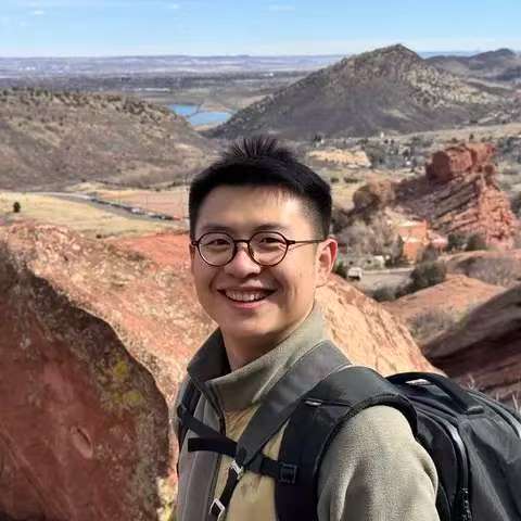
Dr. Ruoyu Wang
Lecturer · Faculty of Engineering, The University of Hong KongDr. Wang is a Lecturer at HKU and holds a Ph.D. in Mechanical and Automation Engineering from CUHK. His research centers on aerial robotics — spanning motion planning, collision-resilient UAV design, and autonomous inspection systems — with publications at top venues like ICRA and IROS. Passionate about experiential engineering education, he mentors the HKUUAS team in designing, building, and iterating real aerial robotic systems from concept to prototype.
Visit BlogSponsor & Recruitment
Partner with us or become a part of the team
Our Sponsors
We are grateful for the generous support from our sponsors who make our research and innovation possible.
Interested in sponsoring us? We'd love to collaborate!
Apply to Join
Scan the QR code below to fill out the application form and join the HKUUAS team!

Scan to apply • We welcome all passionate students!